Stability and Control of Nonlinear Systems
| ✅ Paper Type: Free Essay | ✅ Subject: Engineering |
| ✅ Wordcount: 2317 words | ✅ Published: 30 Aug 2017 |
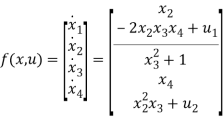
The following system was provided to study about passivity, asymptotic stability, and input to state stability properties at conditions.
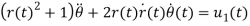
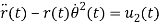
The given system of differential equation for analysis is given below
Also, 
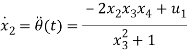
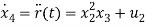
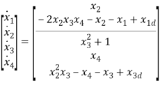
The state space representation of the system is as follows. Let,


Similarly

Hence
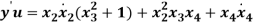
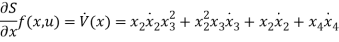
Based on the system equation  is given by

Similarly, based on the state space representation 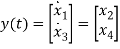
The state of system  , where n=4,
  where m=2 and
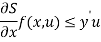
  where p=2. Hence p=m. A dissipative system with respect to supply rate is said to be passive, if
The Lyapunov function for the system is given as
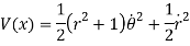
Hence with respect to definition of state variables, it can be rewritten as
Hence,

Also, based on the definition of S,

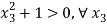
For the given system  , hence the lossless system, is passive from u to y.
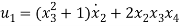
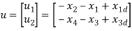
The PD feedback controller of the system with  and
and  is represented as
Hence the state space representation of the system, is given by
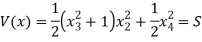
The modified Lyapunov function with potential energy is given by
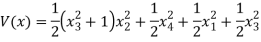
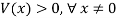
It can be observed that V(x) is differentiable (V: R4 → R and a C1 function).
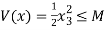
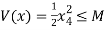
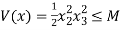
Based on the equation of V(x) it can be observed that,

- The term
 and all other terms are quadratic in nature. Hence
 where
where 
Hence V(x) is positive definite.
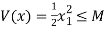
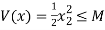
Let V(x) is bounded by V(x)≤M, where M ϵ R, then it implies that
⇒  ⇒
⇒  and
and
⇒  ⇒
⇒  and
and
⇒  ⇒
⇒  and
and
⇒  ⇒
⇒  and
and
⇒  ⇒
⇒ 
Hence V(x) is radially unbounded.
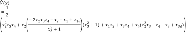
The derivative of V(x) can be obtained as follows

Upon substitution and solving the equations,

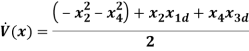
At  It can be observed that
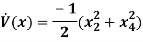
Based on the above equation, it can be observed that
- It can be observed that
 , has only quadratic terms with a negative sign prefixed hence
 where
where 
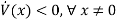
Hence is negative definite.
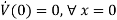
The equilibrium point of the system at  is given by
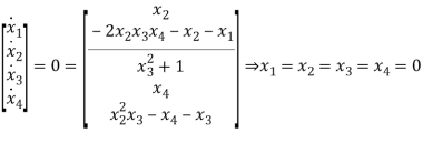
Hence origin is the only equilibrium point of the system.
Based on the above observations, it can be concluded that the system is globally asymptotically stable at the origin.
The given systems were simulated for different values of  and
and  , modified one at a time with other disturbance set to zero and the initial condition set at origin.

The following observations can be found from subplots of  and
and 
Hence the disturbance in both the coordinates of the system are additive in nature. It can be observed that, whenever initial state of the system set to origin and disturbance is induced in one of the coordinate ( or ), the other coordinate of the system is not disturbed.
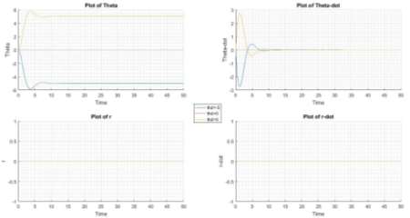
Figure 1 State of System with disturbance at origin with rd=0
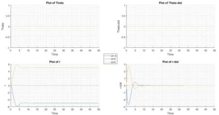
Figure 2 State of System with disturbance at origin with thd=0
The Figure 3 indicates the state of the system, when is modified from -5 to 5 with  , with the initial condition as x = {7,3,5,1}. The settling time of the system varies with the magnitude of disturbance and the initial condition. Also, it can be observed from the plot of that the system settles to a point which is offset from the origin (equilibrium) by the value of disturbance. Also, the settling time of the system is more for d=-c, when compared to d=c. Also, disturbance in one of the coordinate (), has its effect in another coordinate.
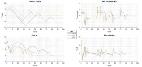
Figure 3 State of System with rd=0 at x = [7,3,5,1]
The observations of disturbance induced in when , is applicable for the disturbance induced in with  Also, it can be observed from Figure 4 that the settling time of the system is higher when a disturbance is induced in r-coordinate, when compared to -coordinate.
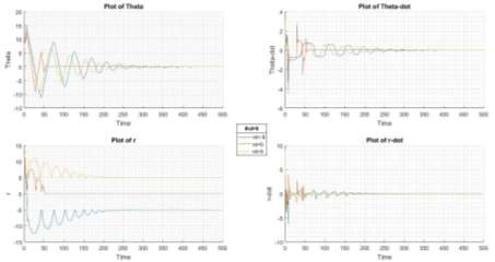
Figure 4 State of System with thd = 0 at x = [7,3,5,1]
The effect of having both and was observed by simulating the system response for  and
and  . Also, it can be observed that settling time of the system is similar to disturbance induced only in the r-coordinate.
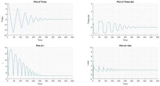
Figure 5 State of System with thd = -5, rd=5 at x = [7,3,5,1]
In all the above plots, it can be observed from the subplot of  that the settling point of state as t→
 ,
,  and
and  , indicating that the state of the system tracks the input in the respective coordinate.
It can also be observed from the previous plots for d=0, system exhibits the property of global asymptotic stability to the origin (equilibrium point). Also,  , the state
  implies the Bounded Input Bounded State property of the system.
The input to state stability of the closed loop system with respect to and for the system was validated by adding a destabilizing feedback with
and  .
.
The function k(x) of the disturbance is selected, such that the power transferred to the system is maximized, which can be performed when  .
.
From the above equation, it can be observed that the power transferred to the system can be maximized by choosing  same sign of
  with c≥0. The nature of system response for different range of ‘c’ is listed in the Table 1 below.
Table 1 System Response for Variation in ‘c’ at initial condition of [7,3,5,1]]
|
Value of c |
Observation |
|
c ≤ 1.99 |
The energy of the system decreases initially, indicated by the plot of Lyapunov function shown in Figure 6 and the same result can be observed on the plot of r and θ, where the magnitude decreases initially and oscillates with the bounded magnitude, for the bounded input indicated in plot of theta-d. |
|
c>1.99 |
For c=5, the energy of the system increases, indicated by the plot of Lyapunov function shown in Figure 7 and the plot of r and θ indicates that the magnitude continues to increases resulting in unbounded state for the bounded input indicated in plot of theta-d. Also, it can be observed that the rate of increase in energy of the system, decreases with time. 
|
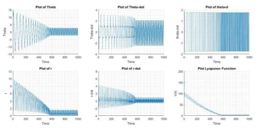
Figure 6 State of System at c=1.75
The system is not Input to state stable (ISS) for c>1.99 and Figure 7 indicates a system which is not ISS for c=5. The value of transition from bounded state to unbounded state was observed at c=1.93 for an initial point of [1,2,1,2]. Based on the above observation, the transition value of c is dependent of initial condition (energy) of the system.
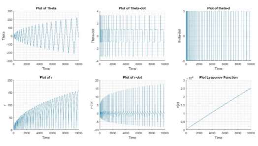
Figure 7 State of System at c=5
The PD control used in the r-coordinate is modified as
The simulations were carried out, to identify the properties of ISS satisfied by the system, with respect to and as inputs. All the simulations were carried out with respect to the initial condition x0 = (7,3,5,1)
Condition 1:
The system is evaluated with zero disturbance  and , the result is indicated in Figure 8.
Figure 8 System with Zero Disturbance
For the no disturbance conditions, it can be observed that the system is asymptotically stable about the origin (equilibrium), indicating the Global asymptotic stability of the system about the origin. Also from the plot of Lyapunov function, it can be observed that the energy of the system settles down to zero.
Condition 2:
The destabilizing feedback input used in question 5 for the system was fed to the system and it its response is indicated in figure

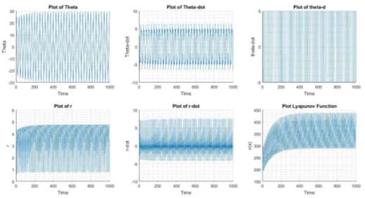
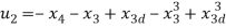
Figure 9 State of System at c=5 with modified PD Control
The following observations can be made with respect to figure
For an input , the state  , indicating bounded input bounded state property of the system. It can be observed that, though the energy of the system increases initially, but upper bounded over a period. The energy and the state of the system gets bounded over period of simulation. Hence for the bounded input, state of the system is bounded. Also, the system exhibits property of asymptotic gain, since the state of the system is upper bounded by disturbance with gain of the system.
Also, it was observed that though the system is ISS for the c=5, as the value of c increases energy of the system increases (example for c=10, v(x) is upper bounded to 10,000). Hence modifying the PD control, makes the system ISS for a larger range of disturbances, when compared to earlier control.
Condition 3:
The system was fed with the input
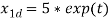
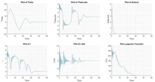
Figure 10 State of system rd=0 and theta d=5*exp(t)
It can be observed from the plot that d(t)→ 0 as  , also
  aysmptotically. Hence the system indicates the property of converging input, converging state.
The response of the system was evaluated with different possible inputs for  , such as

 , the state of the system x1, x3 was chosen based on observations made in earlier simulations (q5) where predominantly these states grew out of bound


Similarly, the above input conditions were simulated with =0 and  defined as one of the input, few combinations of the above input disturbances and few possible system interconnections such as positive feedback interconnection, negative feedback interconnection, series interconnection.
System response for various types of disturbance
- Constant Disturbance
The disturbance of the system is set to constant values, as indicated in Figure 5


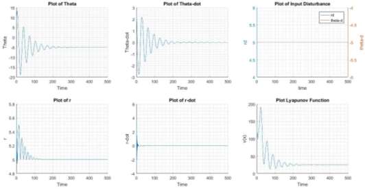
Figure 11 State of system at theta d=-5 rd=5
It can be observed from the plot of Figure 11 and Figure 5 that the settling time of system in r-coordinate has reduced almost by half, when compared to previous control.
- Positive Feedback Interconnection
The disturbance input condition is mentioned below and the system response is shown in Figure 12


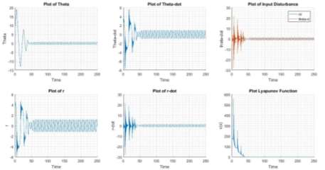
Figure 12 System Response for Positive Feedback Interconnection
The state of the system indicates the converging nature, also it can be observed that after the transient period system follows the input.
- Series Interconnection
The system is connected in series, with the following disturbance input configuration for each of the subsystem and the plot for the same is shown in Figure 13.

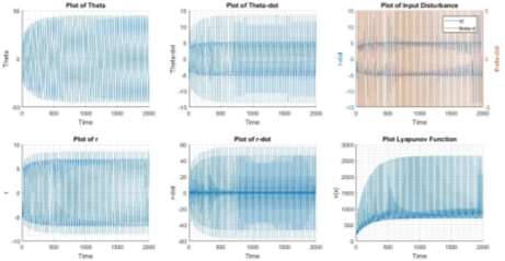
Figure 13 System Response for Series Interconnection
It can be observed that the behavior of the system is similar with respect to condition 2, but the energy of the system settles down at a higher level when compared to the similar condition with 
- System with different disturbances acting simultaneously
The type of disturbance added to the system is given below and the response of the system is shown in figure
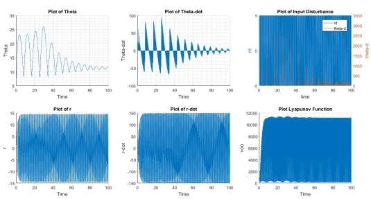
Figure 14 System response of simultaneous time varying disturbance
It can be observed that the system exhibit the property of bounded input bounded state, even if the disturbance is of time varying.
In all the above simulation conditions, it was observed that the system exhibits bounded state nature for a wider range of inputs with higher magnitude, when compared to the PD control implemented earlier. This phenomenon can be attributed to the cubic terms with the negative sign, as it can reduce the rate at which energy of the system increases, before it goes out of bound.
APPENDIX
Code Used for Generation of Plots
Contents
Q4 – Constant Value of Theta-d and r-d
clc
clear all
close all
global x1d;
global x3d;
ts=500; %Duration for solving
ip=[7,3,5,1];
options=odeset(‘AbsTol’,1e-7,’RelTol’,1e-5);
thd=[-5];
rd=[5];
for i=1:size(thd,2)
for j=1:size(rd,2)%-29:30:31
x1d=thd(i); %x1d is Theta-d
x3d=rd(j); %x3d is r-d
[t,x]=ode23(@deeqn,[0 ts],ip,options);
figure(1)
subplot(2,2,1)
hold on
plot(t,x(:,1))
title(‘Plot of Theta’)
xlabel(‘Time’)
ylabel(‘Theta’)
grid on
grid minor
subplot(2,2,2)
hold on
plot(t,x(:,2))
title(‘Plot of Theta-dot’)
xlabel(‘Time’)
ylabel(‘Theta-dot’)
grid on
grid minor
subplot(2,2,3)
hold on
plot(t,x(:,3))
title(‘Plot of r’)
xlabel(‘Time’)
ylabel(‘r’)
grid on
grid minor
subplot(2,2,4)
hold on
plot(t,x(:,4))
title(‘Plot of r-dot’)
xlabel(‘Time’)
ylabel(‘r-dot’)
grid on
grid minor
end
end
Q5 for ISS
clc
close all
global x1d;
global x3d;
ts=10000; %Duration for solving
ip=[7,3,5,1];
options=odeset(‘AbsTol’,1e-7,’RelTol’,1e-5);
x1=ip’;
global c;
cval=[1.92] %1.993 is transition point
for i=1:size(cval,2)
c=cval(i); %4.0125
x1d=0; %x1d is Theta-d
x3d=0; %x3d is r-d
[t,x]=ode23(@deeqnvx,[0 ts],ip,options);
figure(2)
subplot(2,3,1)
hold on
plot(t,x(:,1))
title(‘Plot of Theta’)
xlabel(‘Time’)
ylabel(‘Theta’)
grid on
grid minor
subplot(2,3,2)
hold on
plot(t,x(:,2))
title(‘Plot of Theta-dot’)
xlabel(‘Time’)
ylabel(‘Theta-dot’)
grid on
grid minor
subplot(2,3,4)
hold on
plot(t,x(:,3))
title(‘Plot of r’)
xlabel(‘Time’)
ylabel(‘r’)
grid on
grid minor
subplot(2,3,5)
hold on
plot(t,x(:,4))
title(‘Plot of r-dot’)
xlabel(‘Time’)
ylabel(‘r-dot’)
grid on
grid minor
subplot(2,3,3)
hold on
thdin=c.*sign(x(:,2));
plot(t,thdin)
title(‘Plot of theta-d’)
xlabel(‘Time’)
ylabel(‘theta-dot’)
grid on
grid minor
subplot(2,3,6)
hold on vxfn=(1/2).*(((x(:,3).^2)+1).*(x(:,2).^2)+(x(:,4).^2)+(x(:,1).^2)+(x(:,3).^2));
plot(t,vxfn)
title(‘Plot Lyapunov Function’)
xlabel(‘Time’)
ylabel(‘v(x)’)
grid on
grid minor
end
Q6 for ISS with new u2
clc
close all
global x1d;
global x3d;
ts=100; %Duration for solving
ip=[7,3,5,1];
options=odeset(‘AbsTol’,1e-7,’RelTol’,1e-5);
x1=ip’;
global c;
cval=[5] %1.993 is transition point
for i=1:size(cval,2)
c=cval(i); %4.0125
x1d=0; %x1d is Theta-d
x3d=0; %x3d is r-d
[t,x]=ode23(@deeqnr,[0 ts],ip,options);
figure(3)
subplot(2,3,1)
hold on
plot(t,x(:,1))
title(‘Plot of Theta’)
xlabel(‘Time’)
ylabel(‘Theta’)
grid on
grid minor
subplot(2,3,2)
hold on
plot(t,x(:,2))
title(‘Plot of Theta-dot’)
xlabel(‘Time’)
ylabel(‘Theta-dot’)
grid on
grid minor
subplot(2,3,4)
hold on
plot(t,x(:,3))
title(‘Plot of r’)
Function for constant disturbance
function dx = deeqn(t,x)
% Function for system model
% Argument function for ODE Solver
global x1d;
global x3d;
dx=[x(2); (-2*x(3)*x(4)*x(2)-x(2)-x(1)+x1d)/((x(3).^2)+1);x(4);x(3)*(x(2).^2)-x(4)-x(3)+x3d];
end
System with Destabilizing Feedback
function dx = deeqnvx(t,x)
% Function for system model
% Argument function for ODE Solver
global x1d;
global x3d;
global c;
x1d=c.*sign((+1).*x(2));;
dx=[x(2); (-2*x(3)*x(4)*x(2)-x(2)-x(1)+x1d)/((x(3).^2)+1); x(4); x(3)*(x(2).^2)-x(4)-x(3)+x3d];
end
Function with new u2 and old u1
function dx = deeqnr(t,x)
% Function for system model
% Argument function for ODE Solver
global x1d;
global x3d;
global c;
x1d=x(4);%c.*sign((+1).*x(2));;
x3d=x(2);
dx=[x(2); (-2*x(3)*x(4)*x(2)-x(2)-x(1)+x1d)/((x(3).^2)+1);x(4);x(3)*(x(2).^2)-x(4)-x(3)+x3d-(x(3).^3)+(x3d.^3)];
end
Cite This Work
To export a reference to this article please select a referencing stye below:
Related Services
View all


DMCA / Removal Request
If you are the original writer of this essay and no longer wish to have your work published on UKEssays.com then please click the following link to email our support team:
Request essay removal