Literature Review on Volatility
| ✅ Paper Type: Free Essay | ✅ Subject: Finance |
| ✅ Wordcount: 2114 words | ✅ Published: 04 Sep 2017 |
Literature Review
What is Volatility?
Volatility is defined as the spread of all likely outcomes of an uncertain variable (Poon, 2005). Statistically, it is often measured as the sample standard deviation (as seen below), but can also be measured by variance.
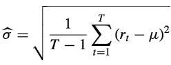
Where rt = return on day t, and
μ = average return over the T-day period.
The common misconception is to equate volatility to risk. However, whilst volatility is related to risk, it is not the same. Risk represents an undesirable outcome, whilst volatility is a measure for uncertainty that could arise from a positive outcome. Furthermore, volatility as a measure for the spread of a distribution contains no information on the shape, this represents another reason for volatility being an imperfect measure for risk. The sole exception to this being a normal distribution or lognormal distribution where mean and standard deviation are appropriate statistics for the whole distribution (Poon, 2005).
In dealing with volatility as a subject matter in financial markets, the focus is on the spread of asset returns. High volatility is generally undesirable as it indicates security values are unreliable and capital markets aren’t functioning efficiently (Poon, 2005; Figlewski, 1997). Financial market volatility has been the subject of much research and the number of studies continues to rise since Poon and Granger (2003)’s original survey first identified 93 papers in the field. A whole host of drivers for volatility have been explored (including political events, macroeconomic factors and investor’s behavior) in an attempt to better capture volatility and decrease risk (Poon, 2005).
This study will add to that list, hoping to contribute something novel to the field by scrutinizing the appropriateness of different volatility models for different country indexes.
The Importance of Volatility Forecasting
- Investment strategies, Portfolio Optimization and Asset Valuation
Volatility when taken as uncertainty transforms into an important component in a wide range of financial applications including Investment strategies for trading or hedging, Portfolio optimization and Asset price valuation. The Markowitz mean-variance portfolio theory (Markowitz, 1952), Capital Asset Pricing Model (Sharpe, 1964) and Sharpe ratio (Sharpe 1966) signify three cornerstones for optimal decision-making and measurement of performance, advocating a focus on the risk-return interrelationship with volatility taken as a risk proxy. With Investors and portfolio managers having limits as to the risk they can bear, accurate forecasts of the volatility of asset prices for long-term horizons is necessary to reliably assess investment risk. Such forecasts allow investors to be better informed and hold stocks for longer rather than constantly reallocating their portfolio in reaction to movements in prices; an often expensive exercise in general (Poon and Granger, 2003). In terms of stock price valuation French, et al. (1987) analyse NYSE common stocks for the period of 1928-1984 and find expected market risk premium to be positively related to the predictable volatility of stock returns, which is further strengthened by the indirect relationship between stock market returns and the unexpected change in the volatility of stock returns.
- Derivatives pricing
Volatility is a key element in Modern option pricing theory that enables estimation of the fair value of options and other derivative instruments. According to Poon and Granger (2003) the trading volume of derivative securities had quadrupled in the recent years leading up to their research and since then this growth has accelerated with the global derivatives market now estimated to be around $544 Trillion excluding credit default swaps and commodity contracts (BIS, 2017). As one of five input variables (including Stock Price, Strike price, time to maturity and risk-free interest rate), expected volatility over the options life in the Black-Scholes model theorized by Black and Scholes (1973) is crucially also the only variable that is not directly observable and must be forecast (Figlewski, 1997). Implied volatility and realized volatility can be computed by referencing observed market prices for options and historical data. Whilst the former is attractive for requiring little input data and delivering excellent results when analysed in some empirical studies compared to time series models utilizing just historical information, it is deficient by not having a firm statistical basis and different strike prices yielding different implied volatilities creating confusion over which implied volatility to use (Tse, 1991; Poon, 2005). Lengthening maturities of derivative instruments also weakens the assumption that volatility realized in the recent past can be used as a fairly reliable proxy for volatility in the near future. (Figlewski, 1997). With recent developments, derivatives written on volatility can now also be purchased whereby volatility represents the underlying asset, thus further necessitating volatility forecasting practices (Poon and Granger, 2003).

- Financial Risk Management
Volatility forecasting plays a significant role in Financial Risk Management of the finance and banking industries. The practice aids in estimation of value-at-risk (VaR), a measure introduced by the Basel Committee in 1996 through an amendment to the Basel Accords (an international standard for minimum capital requirement among international banks to safeguard against various risks). Whilst many risks are examined within, volatility forecasting is most relevant for Market risk and VaR. However, calculating VaR is necessary only if banks choose to adopt its own internal proprietary model for calculating market risk related capital requirement. By choosing to do so, there is greater flexibility for banks in specifying model parameters but with an attached condition of regular backtesting of the internal model. Apart from banks, other financial institutions may also use VaR voluntarily for internal risk management purposes. (Poon and Granger 2003; Poon 2005) Christoffersen and Diebold (2000) do however contend the limits of relevance of Volatility Forecasting for Financial Risk Management, arguing that for reliable forecastablity much depends on whether the horizon of interest is of a short term or long-term nature (taken to be more than 10 or 20 days) with the practice deemed more relevant for the former than the latter due to the limitations in forecastability.
- Policymaking
Financial market volatility can have wide-reaching consequences on economies. As an example, large recessions create ambiguity and hinder public confidence. To counter such negative impacts and disruptions, policy makers utilize market estimates of volatility as a means for identifying the vulnerability of financial markets, equipping them with more reliable and complete information with which to respond with appropriate policies. (Poon and Granger, 2003) The Federal Reserve of the United States is one such entity that incorporates volatility of various financial instruments into its monetary policy decision-making (Nasar, 1991). Bernanke and Gertler (2000) explore the degree to which implications of asset price volatility impact monetary policy decision-making. A side-by-side comparison of U.S. and Japanese monetary policy is the basis of the study. The researchers find that inflation-targeting is desirable, however, monetary policy decisions based on changes in asset prices should only be made to the extent that such changes help to forecast inflationary or deflationary pressures. Meanwhile, Bomfim (2003) investigates the relationship between monetary policy and stock market volatility from the other perspective. Interest rate policy decisions that carry an element of surprise appear to increase short run, stock market volatility significantly with positive surprises also having a greater effect than negative surprises.
Empirical stylized facts of asset returns and volatility
Any attempt to model volatility appropriately must be done with an understanding of the common, recurring set of properties identified from numerous empirical studies carried out across financial instruments, markets and time periods. Contrary to the event-based theory in which it is hypothesized different assets respond differently to different economic and political events, empirical studies show that different assets do in fact share some generalizable, qualitative statistical properties. Volatility models should thus seek to capture these features of asset returns and volatility so as to enhance the forecasting process; herein lays the challenge. (Cont, 2001; Bollerslev et al 1994) Presented are some of these stylized facts, along with their corresponding empirical studies that have contributed to the evolving literature aimed at improving volatility-forecasting practices and which this study will also look to capture.
Return Distributions
Stock Market returns are not normally distributed and it is therefore an unsuitable distribution for modeling returns according to Mandelbrot (1963) and Fama (1965). Returns are approximately symmetrical but can display negative skewness and significantly have leptokurtic features (excess kurtosis with heavier tails and taller, narrower peaks than found in a normal distribution) that see large moves occur with greater frequency than under normal distributions (Sinclair, 2013). Cont (2001) asserts that these large moves in the form of gains and losses are asymmetric by nature with the scale of downward movements in stock index values dwarfing upward movements. He further argues that the introduction of GARCH-type models to counter the effects of volatility clustering can reduce the heaviness of tails in the residual time series to some small extent. However, as GARCH models can at times struggle to fully incorporate heavy-tail features of returns, this has necessitated the use of alternative distributions such as the student’s t-distribution employed in Bollerslev (1987). Alberg et al (2008) employ a skewed version of this distribution to various models with the EGARCH model delivering the best performance in forecasting the volatility of Tel Aviv stock indices. Cont (2001) does however also highlight an important consideration with the notion of aggregational gaussianity that as one increases time scale (t) for calculation of returns, the distribution of returns seems more normally distributed in appearance.
Leverage effect/Asymmetric volatility
In most markets, volatility and returns are negatively correlated (Cont, 2001). First elucidated by Black (1976) and particularly prevalent for stock indices, Volatility will tend to increase when stock price declines. The justification for this is because a decline in equity stock price will increase a company’s debt-to-equity ratio and consequently its risk and volatility (Figlewski and Wang, 2000; Engle and Patton, 2001). Importantly, this relationship is asymmetric, with negative returns having a more marked effect on volatility than positive returns as documented by Christie (1982) and Schwert, (1989). However they also argue that the leverage effect is not enough on its own to explain all of the change in volatility with Christie (1982) incorporating interest rate as another element that has a partial effect. Hence, whilst, ARCH (Engle, 1982) and GARCH (Bollerslev, 1986) models do well to account for volatility clustering and leptokurtosis, their symmetric distribution fails to account for the leverage effect. In response to this, various asymmetric modifications of GARCH have been developed, the most significant of these being Exponential GARCH (EGARCH; Nelson, 1991) and GJR (Glosten et al, 1993). Other models like GARCH-in-Mean have also endeavored to capture the leverage effect along with the risk premium effect, another concept that has been theorized to contribute to volatility asymmetry by studies such as Schwert (1989) (Engle and Patton, 2001).
Volatility Distribution
The distribution of volatility is taken to be approximately log-normal. Various studies such as Andersen et al (2001) have postulated this. More significantly than the actual distribution is the high positive skewness indicating volatility spends longer in lower states than higher states. (Sinclair, 2013)
Volatility-Volume correlation
All measures of volatility and trading volume are highly positively correlated (Cont, 2001). Lee and Rui (2002) show this relationship to be foundationally robust, however what is more complex is determining the causality between the two. Strong arguments can be made either way. As an example, Brooks (1998) utilizes linear and non-linear Granger causality tests and finds the relationship to be stronger from volatility to volume than the converse. He concludes by highlighting that for forecasting accuracy, predicting volume using volatility is more productive than forecasting stock index volume and using such forecasts in trading. According to Gallant et al (1992) this relationship is also closely linked with the leverage effect and incorporating lagged volume weakens the effect considerably.
Non-Constant Volatility
Volatility is not constant. The changing nature of volatility occurs in a particular manner; Merton (1980) was critical of researchers who failed to incorporate this feature in their models. Firstly volatility is mean reverting. Indeed LeBaron (1992) found a strong negative relationship between volatility and autocorrelation for stock indices in the United States. Secondly, Volatility clusters. This is a phenomenon first noted by Mandelbrot (1963) that allows a good estimation of future volatility based on current volatility. Other studies such as Chou (1988) have also empirically shown the existence of clustering. Mandelbrot (1963) wrote, “large changes tend to be followed by large changes of either sign, and small changes tend to be followed by small changes”. In other words, a turbulent day of trading usually comes after another turbulent trading day, whilst a calm period will usually be followed by another calm period. Importantly, the phenomenon is not exclusive to the underlying product and can be seen in stock indices, commodities and currencies. It also tends to be more pronounced in developed than emerging markets. (Taylor, 2008; Sinclair, 2013) Engle and Patton (2001) argue that volatility clustering indicates volatility goes through phases whereby periods of high volatility eventually give way to more normal volatility with the contrary also holding. Engle’s (1982) landmark paper incorporated these features of volatility persistence using his ARCH model, whereby time varying, non-constant volatility that persists in high or low states is taken account of.
Cite This Work
To export a reference to this article please select a referencing stye below:
Related Services
View all


DMCA / Removal Request
If you are the original writer of this essay and no longer wish to have your work published on UKEssays.com then please click the following link to email our support team:
Request essay removal